Error analysis

By default, ScalingProblem estimates an error for every free parameter right after the fit. The keyword error selects the method:

error	the error of a parameter is	accounts for
true, :profile (default)	the displacement at which the quality, re-fitted over the other parameters, reaches error_threshold times its minimum	correlations between the parameters
:conditional	the same, with the other parameters held at their optimum	nothing; smaller or equal to the profile
:bootstrap	the standard deviation of the parameters fitted to n_bootstrap resampled data sets	the error bars of the data
false	not computed (zeros)

Threshold widths: profile and conditional

The quality function has its minimum at the optimal parameters. The profile and conditional methods move one parameter away from its optimum, in both directions, until the quality reaches   (default 1.3). The error is the larger of the two displacements.

• :conditional keeps the other parameters at their optimal values. If the parameters are correlated, the quality rises quickly along this cut, and the error is too small.

• :profile re-fits the other parameters at every displacement, i.e. it follows the valley of the quality function. With one free parameter, both methods agree.

The difference is easiest to see in the quality landscape of two correlated parameters. We fit synthetic data with error bars ( ,  ):

using ScalingCollapse
using Random

F(z) = 1 / (1 + exp(z)) + 0.3 * tanh(z)^2
Ls = [16, 32, 64, 128]
xs = collect(range(0.9, 1.1; length=41))
rng = Xoshiro(2)
ys = Vector{Float64}[]
es = Vector{Float64}[]
for L in Ls
    y = F.((xs .- 1.0) .* L^(1 / 0.8))
    e = fill(0.01, length(xs))
    push!(ys, y .+ e .* randn(rng, length(y)))
    push!(es, e)
end

sp = ScalingProblem(xs, ys, es, Ls;
    sf=ScalingFunction(:x; p_names=["x_c", "nu"]),
    p_space=[0.95:0.005:1.05, 0.4:0.1:1.6],
    dx=[-1.0, 3.0],
)

ScalingProblem
    Scaling function:
        x -> (x - x_c) * L^(1/nu)
        y -> y
    Optimal parameters:
        x_c = 0.9997731574541192 ± 0.0003007106262075519
        nu = 0.8131509031302264 ± 0.04765214351797969
    Optimization interval dx:
        -1.0 < x < 3.0
    Searched parameter space:
        x_c ∈ 0.95:0.005:1.05
        nu ∈ 0.4:0.1:1.6

parameter_errors computes the errors of a solved problem with another method, without changing it:

σ_profile = sp.optimal_ps_error
σ_conditional = parameter_errors(sp; method=:conditional)
σ_bootstrap = parameter_errors(sp; method=:bootstrap, n_bootstrap=200, rng=Xoshiro(1))
[σ_profile σ_conditional σ_bootstrap]

2×3 Matrix{Float64}:
 0.000300711  0.000238242  0.000101552
 0.0476521    0.03673      0.0138282

residuals evaluates the quality on a grid around the optimum (by default errors in every parameter). The dashed line is the threshold  : the profile error is the extent of this contour along an axis, the conditional error the extent of the cut through the optimum. The bootstrap error is unrelated to the threshold.

using CairoMakie

ps, S = residuals(sp; N_steps=81)
x_c, nu = sp.optimal_ps

fig = Figure(size=(620, 460))
ax = Axis(fig[1, 1]; xlabel=L"x_c", ylabel=L"\nu", title="quality landscape")
hm = heatmap!(ax, ps[1], ps[2], log10.(S ./ sp.minimum); colormap=:Blues)
contour!(ax, ps[1], ps[2], S ./ sp.minimum; levels=[1.3], color=:black, linewidth=1.5,
    linestyle=:dash)
Colorbar(fig[1, 2], hm; label=L"\log_{10}(S / S_\mathrm{min})")

# error bars through the optimum, from the widest to the narrowest
colors = Makie.wong_colors()
for (σ, label, color, width) in ((σ_profile, "profile", :black, 6),
    (σ_conditional, "conditional", colors[1], 4), (σ_bootstrap, "bootstrap", colors[2], 2))
    lines!(ax, [x_c - σ[1], x_c + σ[1]], [nu, nu]; color, linewidth=width, label)
    lines!(ax, [x_c, x_c], [nu - σ[2], nu + σ[2]]; color, linewidth=width)
end
scatter!(ax, [x_c], [nu]; color=:white, strokecolor=:black, strokewidth=1.5, markersize=10)
axislegend(ax; position=:rb)
fig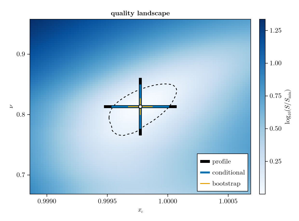

What the threshold widths mean

Profile and conditional errors are widths defined by a threshold on the quality, not standard deviations with a known coverage. The quality is quadratic around its minimum, so the width grows as with the threshold : halving the error takes   instead of 1.3. Change the threshold with error_threshold (one number, or one per free parameter).

The default 1.3 is a convention. In a benchmark on synthetic data with known parameters (about 3700 fits of monotone curves and peaks, with and without error bars):

• If the data deviate from scaling only by noise, the widths are about 4 times the statistical error, i.e. the scatter of the fitted parameters between independent noisy data sets. A threshold of about  , with the number of data points in the overlap window, would match it. Since the default is a fixed ratio, the widths do not shrink when more points are added.

• With corrections to scaling, the deviation from the true parameters is often larger than the statistical error. On the test cases with exactly known parameters, the deviations at 1.3 are typically about one width, and up to about four.

So the default widths are a conservative estimate of the statistical error and of the order of the systematic deviation of typical data, but no bound on it. They are useful to compare fits and to judge how well the data constrain a parameter. For a statistical error, use error=:bootstrap (needs error bars).

When the profile finds a better fit

The profile re-fits the other parameters at every displacement. If one of these fits finds a lower quality than minimum inside p_space, the original fit was not at the minimum. The constructor (and parameter_errors!) then re-optimizes from there, with a warning, and restarts the analysis, up to three times; optimal_ps and minimum change accordingly. parameter_errors throws an error instead, since it does not change the problem.

When an error is NaN

An error is NaN, with a warning that names the reason, if

• the quality never reaches the threshold on one side (within 60 outward steps),

• the quality becomes undefined first, because the rescaled data no longer overlap within dx,

• the profile finds a lower quality outside p_space: widen p_space,

• the re-optimizations of the profile run out (then all errors are NaN).

Bootstrap errors

With error bars, error=:bootstrap estimates statistical errors: it draws n_bootstrap synthetic data sets in which every y value is replaced by a Gaussian random number centered on it, with its error bar as width, fits each of them (starting from optimal_ps), and reports the standard deviation of the fitted parameters.

using Random
ScalingProblem(xs, ys, es, Ls;
    sf=ScalingFunction(:x; p_names=["x_c", "nu"]),
    error=:bootstrap, n_bootstrap=500, rng=Xoshiro(1),
)

• It costs about n_bootstrap fits. Its errors scatter between random seeds by a relative amount of about , i.e. 7% for the default of 100 samples, enough for one significant digit; use 500 or more for a reliable second digit.

• Pass a seeded random number generator rng for reproducible errors.

• It assumes independent Gaussian errors, and it only captures the statistical noise of the data. Systematic deviations from the scaling form, e.g. corrections to scaling, are not part of it. In the example above, the bootstrap errors are much smaller than the threshold widths; the percolation example shows a case where the true values lie far outside the bootstrap errors.

• optimal_ps and minimum remain those of the original data.

Computing errors after the fit

Fitting with error=false skips the error analysis, which is useful while exploring. parameter_errors then computes errors with any method, without changing the problem; its keywords default to the settings of the problem. parameter_errors! does the same, but stores the errors and settings in the problem:

sp_fast = ScalingProblem(xs, ys, es, Ls;
    sf=ScalingFunction(:x; p_names=["x_c", "nu"]),
    p_space=[0.95:0.005:1.05, 0.4:0.1:1.6],
    dx=[-1.0, 3.0],
    error=false,
)
parameter_errors!(sp_fast; method=:profile)
sp_fast

ScalingProblem
    Scaling function:
        x -> (x - x_c) * L^(1/nu)
        y -> y
    Optimal parameters:
        x_c = 0.9997731574541192 ± 0.0003007106262075519
        nu = 0.8131509031302264 ± 0.04765214351797969
    Optimization interval dx:
        -1.0 < x < 3.0
    Searched parameter space:
        x_c ∈ 0.95:0.005:1.05
        nu ∈ 0.4:0.1:1.6