Getting Started

This tutorial performs a complete finite-size scaling analysis of synthetic data whose critical parameters we know, so that we can check the result. The examples apply the same steps to real data.

The data

Suppose we measured an order parameter at the control parameter (e.g. a temperature) for four system sizes , each point with an error bar. We generate such data from the scaling form

with  ,   and  , and add 1% Gaussian noise:

using ScalingCollapse
using Random

x_c, ν, β = 0.5, 1.2, 0.3
F(z) = 1 / (1 + exp(2z)) + 0.2       # the master curve

rng = Xoshiro(42)
Ls = [16, 32, 64, 128]
xs = collect(range(0.3, 0.7; length=41))
ys = Vector{Float64}[]
es = Vector{Float64}[]
for L in Ls
    y = L^(-β / ν) .* F.((xs .- x_c) .* L^(1 / ν))
    e = 0.01 .* y                    # error bars
    push!(ys, y .+ e .* randn(rng, length(y)))
    push!(es, e)
end

All sizes share the x values xs, so a single vector is enough; ys and es hold one vector per system size. Input data lists all accepted formats, including matrices and Measurements.

Solving the scaling problem

A ScalingProblem needs the data, a ScalingFunction that describes the scaling form, and a range for each parameter to search:

sp = ScalingProblem(xs, ys, es, Ls;
    sf=ScalingFunction(:xy; p_names=["x_c", "nu", "beta"]),
    p_space=[0.4:0.01:0.6, 0.5:0.1:2.0, 0.0:0.05:0.6],
    dx=[-3.0, 3.0],
)

ScalingProblem
    Scaling function:
        x -> (x - x_c) * L^(1/nu)
        y -> y * L^(beta/nu)
    Optimal parameters:
        x_c = 0.4993633106128095 ± 0.0010700319582023143
        nu = 1.199966497848909 ± 0.026560857304822175
        beta = 0.2966346416241594 ± 0.012373184632310142
    Optimization interval dx:
        -3.0 < x < 3.0
    Searched parameter space:
        x_c ∈ 0.4:0.01:0.6
        nu ∈ 0.5:0.1:2.0
        beta ∈ 0.0:0.05:0.6

The constructor did all the work:

1. The preset :xy rescales the data as    and   ; p_names gives the three parameters their names.

2. It evaluated the quality of the collapse on every point of the grid p_space and refined the best candidates with the Nelder–Mead method.

3. It estimated the error of every parameter (by default from the profile of the quality function, see Error analysis).

dx restricts the comparison of the curves to rescaled x values between -3 and 3, i.e. to the critical region, where the scaling form holds best. All three parameters agree with the values we put in. The results are fields of sp:

sp.optimal_ps

3-element Vector{Float64}:
 0.4993633106128095
 1.199966497848909
 0.2966346416241594

sp.optimal_ps_error

3-element Vector{Float64}:
 0.0010700319582023143
 0.026560857304822175
 0.012373184632310142

sp.minimum # the quality of the collapse at the optimum (lower is better)

0.5051654376586426

Plotting the collapse

scaled_data returns the rescaled data, one vector per system size. Plotted next to the raw data, the collapse looks like this (the dashed lines mark the window dx):

using CairoMakie

xs_scaled, ys_scaled, es_scaled, _ = scaled_data(sp)

colors = cgrad(:Blues)[range(0.35, 1.0; length=length(Ls))]
fig = Figure(size=(760, 320))
ax1 = Axis(fig[1, 1]; xlabel=L"x", ylabel=L"Y", title="data")
ax2 = Axis(fig[1, 2]; xlabel=L"(x - x_c)\,L^{1/\nu}", ylabel=L"Y\,L^{\beta/\nu}",
    title="collapse")
for i in eachindex(Ls)
    errorbars!(ax1, xs, ys[i], es[i]; color=colors[i])
    scatter!(ax1, xs, ys[i]; color=colors[i], markersize=6, label="L = $(Ls[i])")
    errorbars!(ax2, xs_scaled[i], ys_scaled[i], es_scaled[i]; color=colors[i])
    scatter!(ax2, xs_scaled[i], ys_scaled[i]; color=colors[i], markersize=6)
end
vlines!(ax2, sp.dx; color=:gray, linestyle=:dash)
xlims!(ax2, -8, 8)
Legend(fig[1, 3], ax1)
fig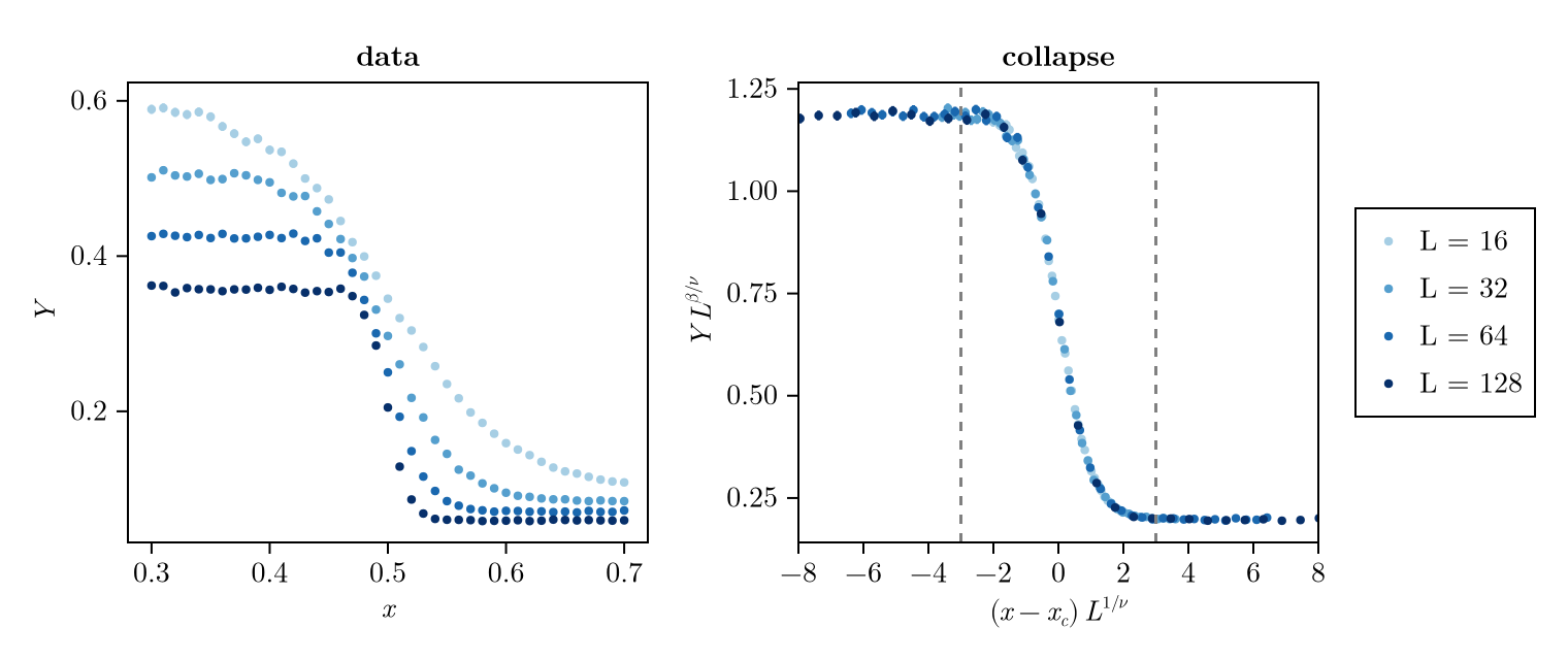

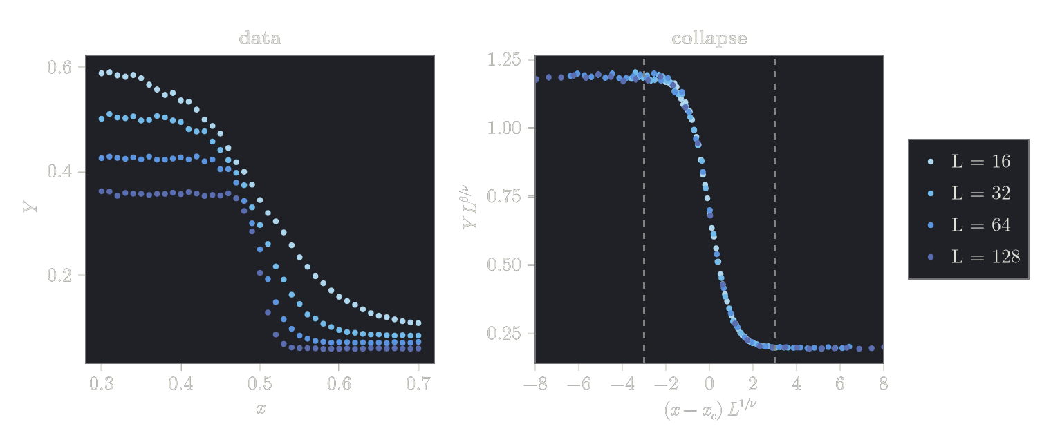
Figure style

The figures in this documentation use LaTeX fonts and no grid lines. To get the same style, run set_theme!(theme_latexfonts(); Axis=(xgridvisible=false, ygridvisible=false)) once before plotting.

Fixing a parameter

If a parameter is known, e.g. from theory, fix it by passing its name and value to the ScalingFunction. It is then no longer fitted, and p_space, optimal_ps and optimal_ps_error only refer to the remaining free parameters:

sp_fixed = ScalingProblem(xs, ys, es, Ls;
    sf=ScalingFunction(:xy; p_names=["x_c", "nu", "beta"], nu=1.2),
    p_space=[0.4:0.01:0.6, 0.0:0.05:0.6],
    dx=[-3.0, 3.0],
)

ScalingProblem
    Scaling function:
        x -> (x - x_c) * L^(1/nu)
        y -> y * L^(beta/nu)
    Fixed parameters:
        nu = 1.2
    Optimal parameters:
        x_c = 0.49936275917764916 ± 0.0009338774869884483
        beta = 0.29664095379804645 ± 0.011326437393130226
    Optimization interval dx:
        -3.0 < x < 3.0
    Searched parameter space:
        x_c ∈ 0.4:0.01:0.6
        beta ∈ 0.0:0.05:0.6

Next steps

• Finite-size scaling explains which preset fits which observable.

• Fitting covers the search (p_space, starting_ps, dx) and what to do when a fit fails.

• Error analysis compares the error methods and shows how to inspect the quality landscape.

• The examples start with the 2D Ising model.