Uniform grids and quality landscapes

A fit is only as good as the quality function it minimizes. This example uses residuals to look at the quality landscape of all quality functions, and shows why the default MultipleSplines is smooth where the others are not.

The data

We use the spanning probability of bond percolation on the square lattice ( ,  ), computed with the Newman–Ziff algorithm for   to , with error bars. The data are in test/testdata/percolation of the repository. The probabilities were chosen on a grid that is uniform in the scaling variable   , a common choice to place the same number of points in the critical region of every size.

using ScalingCollapse
using HDF5

file = joinpath(pkgdir(ScalingCollapse), "test", "testdata", "percolation", "bond_square.h5")
Ls, xs, ys, es = h5open(file) do h
    Ls = read(h, "Ls")
    curves(v) = [read(h, "spanning/L$L/$v") for L in Ls]  # one vector per size
    Ls, curves("x"), curves("y"), curves("e")
end

Fits with every quality function

sf = ScalingFunction(:x; p_names=["p_c", "nu"])
setup = (; sf, p_space=[0.48:0.002:0.52, 0.8:0.1:2.0], dx=[-0.5, 0.5])
qualities = ["MultipleSplines" => MultipleSplines(), "Linear" => Linear(),
    "SingleSpline" => SingleSpline(), "Houdayer" => Houdayer()]
fits = [name => ScalingProblem(xs, ys, es, Ls; setup..., quality) for (name, quality) in qualities]
for (name, sp) in fits
    println(rpad(name, 16), "p_c = ", round(sp.optimal_ps[1]; digits=5), " ± ",
        round(sp.optimal_ps_error[1]; digits=5), ",  nu = ", round(sp.optimal_ps[2]; digits=3),
        " ± ", round(sp.optimal_ps_error[2]; digits=3))
end

MultipleSplines p_c = 0.50074 ± 0.00036,  nu = 1.319 ± 0.045
Linear          p_c = 0.50069 ± 0.00036,  nu = 1.318 ± 0.043
SingleSpline    p_c = 0.50079 ± 0.00038,  nu = 1.319 ± 0.048
Houdayer        p_c = 0.50097 ± 0.00042,  nu = 1.313 ± 0.046

All four fits agree with each other, and with the exact values to within about two errors. Their landscapes do not.

The landscapes

residuals evaluates the quality function of a problem on a parameter grid. We plot on the same grid for every quality function:

using CairoMakie

grid = [0.497:0.0001:0.503, 1.0:0.005:1.7]
fig = Figure(size=(780, 620))
for (k, (name, sp)) in enumerate(fits)
    ps, S = residuals(sp; p_space=grid)
    ax = Axis(fig[fldmod1(k, 2)...]; title=name, xlabel=L"p_c", ylabel=L"\nu")
    heatmap!(ax, ps[1], ps[2], log10.(S ./ minimum(S));
        colormap=Reverse(:Blues), colorrange=(0, 1.5))
    scatter!(ax, [0.5], [4 / 3]; color=:white, strokecolor=:black, strokewidth=1.5,
        markersize=10)
end
Colorbar(fig[1:2, 3]; colormap=Reverse(:Blues), colorrange=(0, 1.5),
    label=L"\log_{10}(S / S_\mathrm{min})")
fig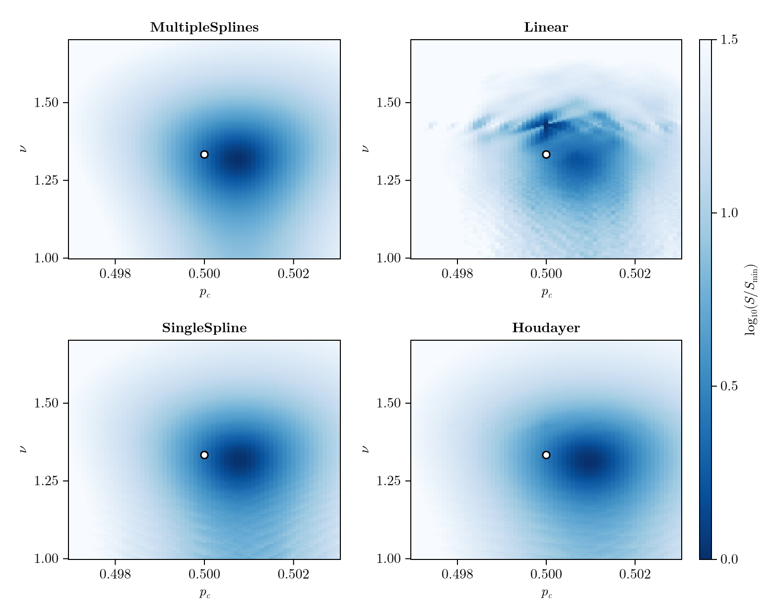

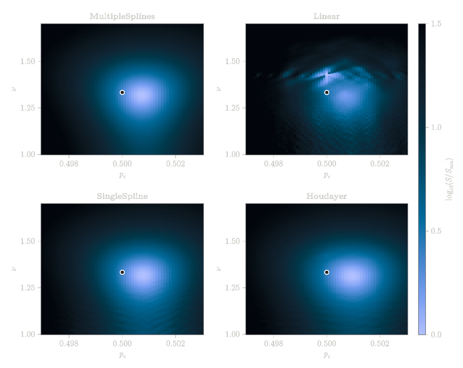
The white dot marks the exact values. MultipleSplines has a single smooth valley close to them. SingleSpline and Houdayer are rippled, and Linear has a sharp cross-shaped structure at  ,  .

A cut along at the exact   shows what happens there:

fig = Figure(size=(780, 360))
ax = Axis(fig[1, 1]; xlabel=L"\nu", ylabel=L"S / S_\mathrm{min}", yscale=log10,
    yticks=[1, 2, 5, 10, 20, 50], title=L"quality at $p_c = 1/2$")
for (name, sp) in fits
    ps, S = residuals(sp; dims=[1, 2], p_space=[0.5:0.5, 1.0:0.002:1.8])
    lines!(ax, ps[2], S[1, :] ./ minimum(S); linewidth=2, label=name)
end
vlines!(ax, [4 / 3, 1 / 0.7]; color=:gray, linestyle=:dash)
Legend(fig[1, 2], ax)
fig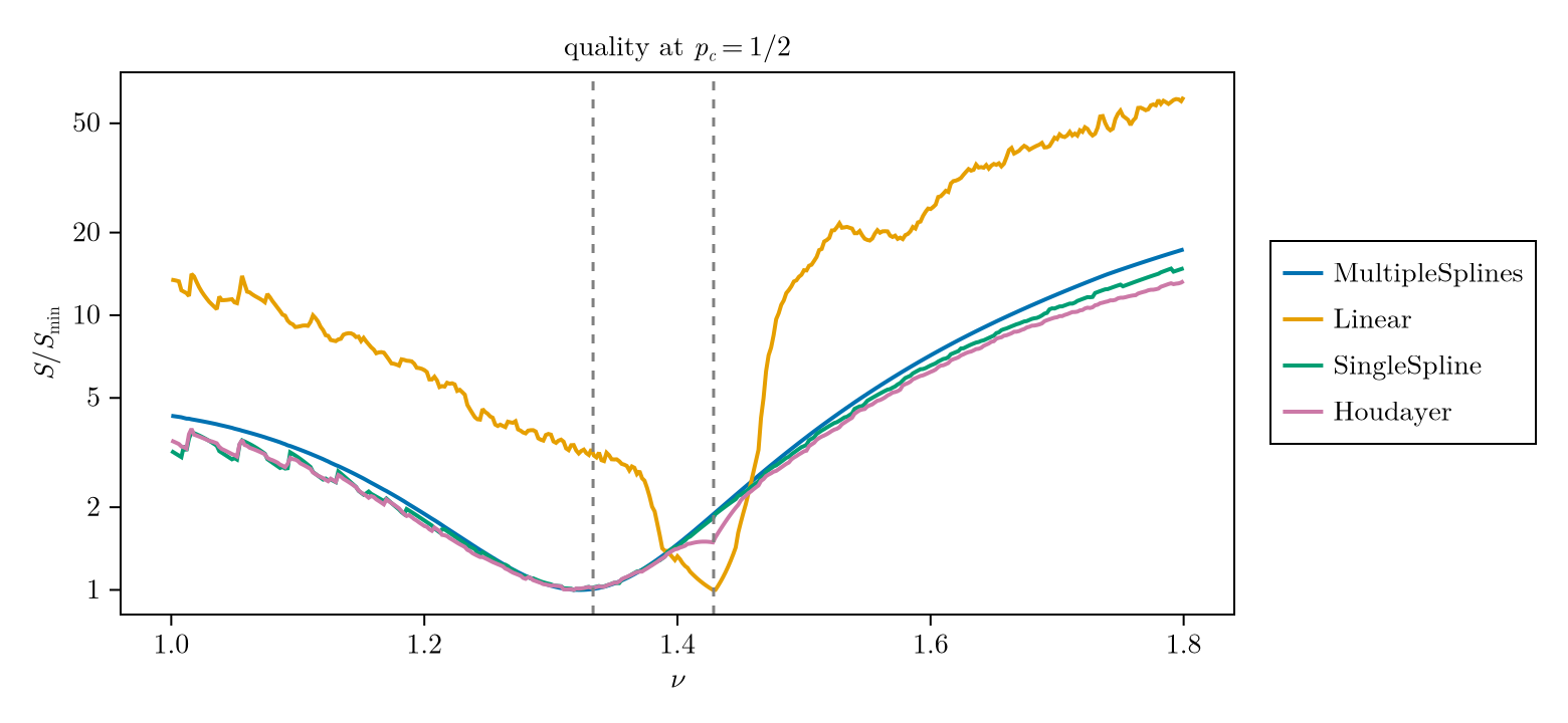

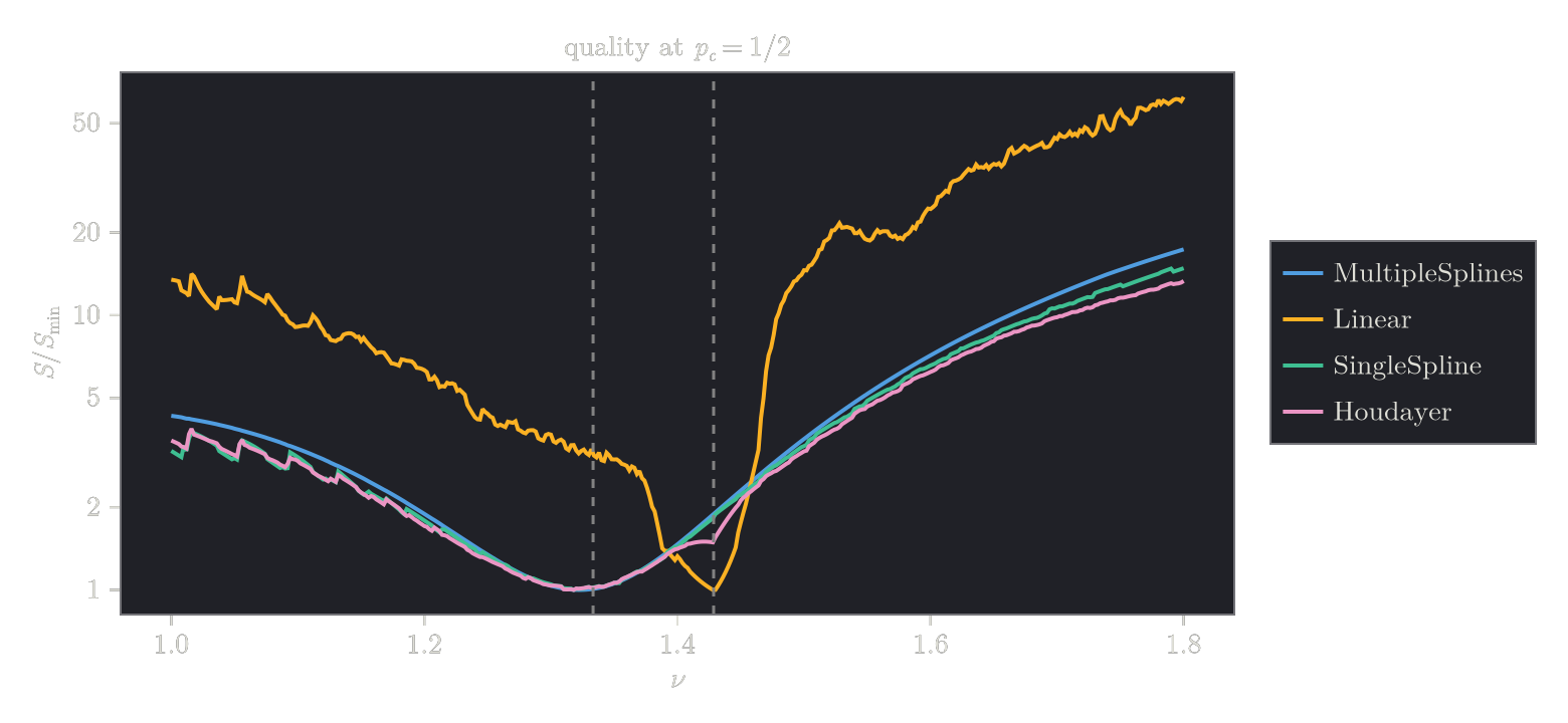
The dashed lines mark   and  . At   and  , the rescaled x values of all sizes coincide, because the data grid is uniform in  . Linear then compares points of different sizes at the same x, without any interpolation error, and its quality drops to a false minimum, lower than the one near the true . The quality functions that compare individual points (Linear, SingleSpline, Houdayer) also jump whenever points of different sizes pass each other, which produces the ripples.

MultipleSplines compares smooth interpolations of every size on a fixed set of points, so it does not care how the grids of the sizes line up. Its landscape is smooth, which makes both the fit and the error analysis reliable.

Tip

Whatever the quality function, plotting the landscape around a fit with residuals is a quick check that the minimum is real and not an artifact of the data grid.