Site percolation with error bars

Site percolation on the square lattice has a percolation threshold   (known numerically to high precision) and the exact exponents   and  . We analyze the order parameter, the relative size of the largest cluster, for   to , with error bars. The data are the example data of autoScale.py by O. Melchert (MIT license), shipped in test/testdata/autoscale of the repository.

This example shows how to use error bars, how corrections to scaling show up, and how the error methods differ.

The data

Every file has three columns: occupation probability , order parameter and its error. Lines starting with # are comments.

using ScalingCollapse
using DelimitedFiles

dir = joinpath(pkgdir(ScalingCollapse), "test", "testdata", "autoscale")
Ls = [8, 16, 32, 64, 128, 256, 512]
tables = [readdlm(joinpath(dir, "orderParam_L$L.dat"); comments=true) for L in Ls]
ps = [t[:, 1] for t in tables]   # occupation probability
P = [t[:, 2] for t in tables]    # order parameter
Pe = [t[:, 3] for t in tables]   # its error
length.(ps)

7-element Vector{Int64}:
 31
 33
 33
 44
 43
 44
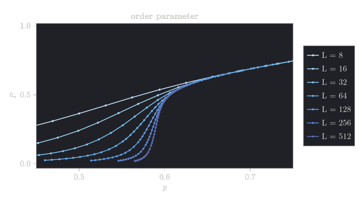
 44

The sizes are measured at different values of and with different numbers of points, so all inputs are vectors of vectors. The error bars Pe are passed as the fourth argument.

using CairoMakie

colors = cgrad(:Blues)[range(0.3, 1.0; length=length(Ls))]
fig = Figure(size=(620, 340))
ax = Axis(fig[1, 1]; xlabel=L"p", ylabel=L"P", title="order parameter")
for i in eachindex(Ls)
    errorbars!(ax, ps[i], P[i], Pe[i]; color=colors[i])
    scatterlines!(ax, ps[i], P[i]; color=colors[i], markersize=5, label="L = $(Ls[i])")
end
xlims!(ax, 0.45, 0.75)
Legend(fig[1, 2], ax)
fig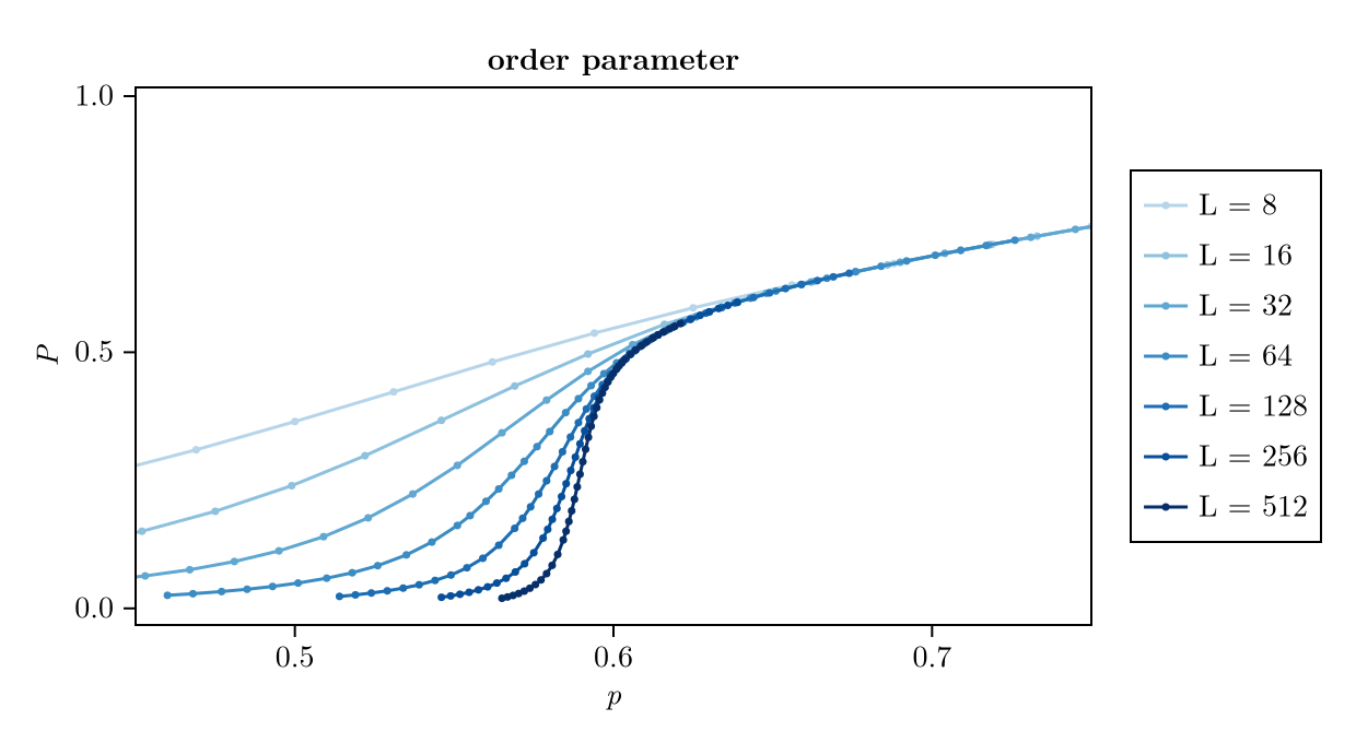

Fit with all sizes

The order parameter scales as   , the preset :xy. We restrict the fit to the window     around the threshold:

sf = ScalingFunction(:xy; p_names=["p_c", "nu", "beta"])
p_space = [0.58:0.002:0.61, 0.8:0.1:2.0, 0.05:0.025:0.3]
dx = [-1.5, 1.0]

sp_all = ScalingProblem(ps, P, Pe, Ls; sf, p_space, dx)

ScalingProblem
    Scaling function:
        x -> (x - p_c) * L^(1/nu)
        y -> y * L^(beta/nu)
    Optimal parameters:
        p_c = 0.5916813894963331 ± 0.0006322587227533402
        nu = 1.2985252861016483 ± 0.03633395866561683
        beta = 0.15869698207951638 ± 0.00819883023280881
    Optimization interval dx:
        -1.5 < x < 1.0
    Searched parameter space:
        p_c ∈ 0.58:0.002:0.61
        nu ∈ 0.8:0.1:2.0
        beta ∈ 0.05:0.025:0.3

The collapse looks convincing, yet and lie several errors away from the exact values.

Corrections to scaling

The scaling form only holds for large . A simple check is to drop the smallest sizes one after the other and watch whether the parameters drift:

L_mins = Ls[1:5]
fits = [ScalingProblem(ps[k:end], P[k:end], Pe[k:end], Ls[k:end]; sf, p_space, dx)
        for k in eachindex(L_mins)]

exact = [0.5927460508, 4 / 3, 5 / 36]
labels = [L"p_c", L"\nu", L"\beta"]
fig = Figure(size=(780, 280))
for j in 1:3
    ax = Axis(fig[1, j]; xlabel=L"L_\mathrm{min}", ylabel=labels[j], xscale=log2,
        xticks=L_mins)
    hlines!(ax, [exact[j]]; color=:gray, linestyle=:dash)
    v = [f.optimal_ps[j] for f in fits]
    σ = [f.optimal_ps_error[j] for f in fits]
    errorbars!(ax, L_mins, v, σ; color=:black, whiskerwidth=6)
    scatter!(ax, L_mins, v; color=:black, markersize=8)
end
fig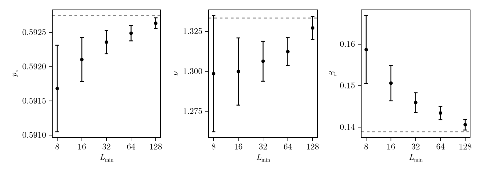

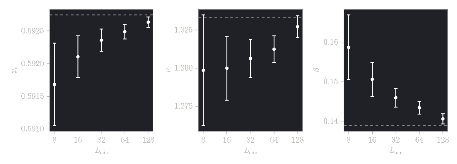
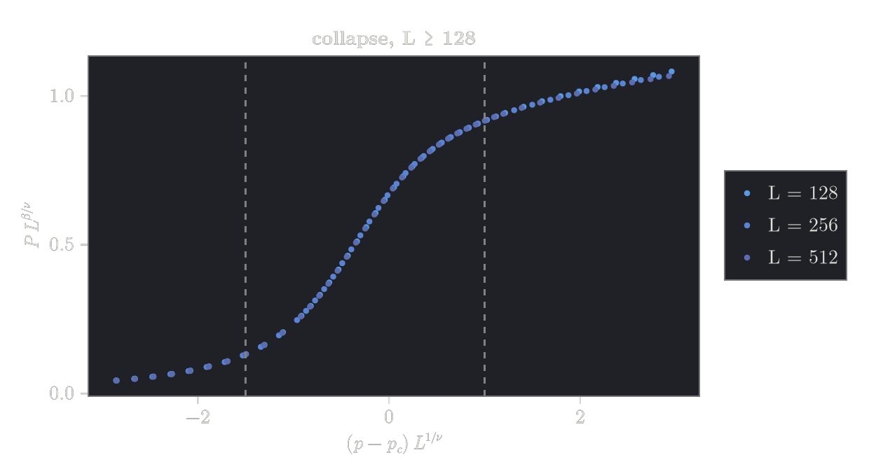
The estimates move steadily towards the exact values (dashed) as the smallest sizes are removed. With  , all three agree with them within about two errors:

sp = fits[end]

ScalingProblem
    Scaling function:
        x -> (x - p_c) * L^(1/nu)
        y -> y * L^(beta/nu)
    Optimal parameters:
        p_c = 0.5926349851950006 ± 7.933097685228381e-5
        nu = 1.3271383611181755 ± 0.00716104851550221
        beta = 0.14060129773112817 ± 0.0012798854058588985
    Optimization interval dx:
        -1.5 < x < 1.0
    Searched parameter space:
        p_c ∈ 0.58:0.002:0.61
        nu ∈ 0.8:0.1:2.0
        beta ∈ 0.05:0.025:0.3

xs_s, ys_s, es_s, _ = scaled_data(sp)
fig = Figure(size=(620, 340))
ax = Axis(fig[1, 1]; xlabel=L"(p - p_c)\,L^{1/\nu}", ylabel=L"P\, L^{\beta/\nu}",
    title="collapse, L ≥ 128")
for (i, L) in enumerate(Ls[5:end])
    inside = -3 .<= xs_s[i] .<= 3
    c = colors[4+i]
    errorbars!(ax, xs_s[i][inside], ys_s[i][inside], es_s[i][inside]; color=c)
    scatter!(ax, xs_s[i][inside], ys_s[i][inside]; color=c, markersize=6, label="L = $L")
end
vlines!(ax, dx; color=:gray, linestyle=:dash)
Legend(fig[1, 2], ax)
fig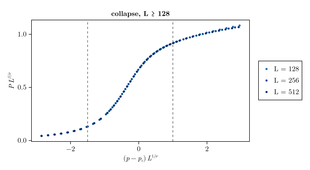

Profile and bootstrap errors

With error bars, error=:bootstrap gives the statistical errors of the parameters: the spread of fits to data sets resampled within the error bars.

using Random

for (name, s) in ("all sizes" => sp_all, "L ≥ 128" => sp)
    σ_boot = parameter_errors(s; method=:bootstrap, n_bootstrap=200, rng=Xoshiro(1))
    println(name)
    for j in 1:3
        p = ScalingCollapse.scaled_p_names(sf)[j]
        println("    ", rpad(p, 5), "deviation from exact ",
            rpad(round(s.optimal_ps[j] - exact[j]; sigdigits=2), 10),
            "profile ", rpad(round(s.optimal_ps_error[j]; sigdigits=2), 9),
            "bootstrap ", round(σ_boot[j]; sigdigits=2))
    end
end

all sizes
    p_c  deviation from exact -0.0011   profile 0.00063  bootstrap 1.7e-5
    nu   deviation from exact -0.035    profile 0.036    bootstrap 0.001
    beta deviation from exact 0.02      profile 0.0082   bootstrap 0.00021
L ≥ 128
    p_c  deviation from exact -0.00011  profile 7.9e-5   bootstrap 3.0e-5
    nu   deviation from exact -0.0062   profile 0.0072   bootstrap 0.0031
    beta deviation from exact 0.0017    profile 0.0013   bootstrap 0.00048

The bootstrap errors are several times smaller than the profile widths, and for all sizes the deviations from the exact values exceed them by more than an order of magnitude: the bootstrap measures the noise of the data, not the systematic error of an incomplete scaling form. Quote bootstrap errors only after checking for corrections to scaling as above. The profile widths are not calibrated either, but they are a more conservative measure of how well the data constrain the parameters.