Mean-field model: exact data

The Curie–Weiss model couples all Ising spins with each other, with the energy    of the total magnetization . It is the mean-field limit of the Ising model, with   and the mean-field exponents   and  . The role of the system size is played by , and the scaling variable is  , so the exponent nu of the presets is  .

For this model, the partition function is a sum over the   values of , so the observables of a finite system can be computed exactly. This example computes them on the fly and fits noise-free data.

Exact finite-size data

using ScalingCollapse

# probabilities of the magnetization per spin m = M/N at temperature T
function distribution(N, T)
    logw = zeros(N + 1)            # log binomial(N, k), by recursion over k
    for k in 0:N-1
        logw[k+2] = logw[k+1] + log((N - k) / (k + 1))
    end
    Ms = [2k - N for k in 0:N]
    logw .+= Ms .^ 2 ./ (2N * T)   # Boltzmann weight exp(M²/(2NT))
    w = exp.(logw .- maximum(logw))
    return Ms ./ N, w ./ sum(w)
end

# Binder cumulant and susceptibility
function observables(N, T)
    m, w = distribution(N, T)
    m1, m2, m4 = sum(w .* abs.(m)), sum(w .* m .^ 2), sum(w .* m .^ 4)
    return 1 - m4 / (3m2^2), N * (m2 - m1^2) / T
end

Ns = [256, 1024, 4096, 16384]
Ts = collect(range(0.9, 1.1; length=41))
obs = [observables.(N, Ts) for N in Ns]
U = [first.(o) for o in obs]
chi = [last.(o) for o in obs]

Binder cumulant

For noise-free data, cubic splines interpolate more accurately than the default monotone interpolation, so we use MultipleSplines(interp=:cubic) (see Quality functions):

sp_U = ScalingProblem(Ts, U, Ns;
    sf=ScalingFunction(:x; p_names=["T_c", "nu"]),
    p_space=[0.9:0.01:1.1, 1.0:0.1:3.0],
    dx=[-2.0, 2.0],
    quality=MultipleSplines(interp=:cubic),
)

ScalingProblem
    Scaling function:
        x -> (x - T_c) * L^(1/nu)
        y -> y
    Optimal parameters:
        T_c = 0.9989974399979069 ± 0.00041363100859527
        nu = 1.9829418226820394 ± 0.05841166223464751
    Optimization interval dx:
        -2.0 < x < 2.0
    Searched parameter space:
        T_c ∈ 0.9:0.01:1.1
        nu ∈ 1.0:0.1:3.0

Susceptibility

The susceptibility    has a peak that grows as , the preset :xny:

sp_chi = ScalingProblem(Ts, chi, Ns;
    sf=ScalingFunction(:xny; p_names=["T_c", "nu", "gamma"]),
    p_space=[0.9:0.01:1.1, 1.0:0.1:3.0, 0.5:0.1:1.5],
    dx=[-1.0, 1.0],
    quality=MultipleSplines(interp=:cubic),
)

ScalingProblem
    Scaling function:
        x -> (x - T_c) * L^(1/nu)
        y -> y * L^(-gamma/nu)
    Optimal parameters:
        T_c = 0.9994342215950882 ± 0.0002032011285825485
        nu = 2.0052423285269594 ± 0.01888288249567487
        gamma = 1.0318872876514056 ± 0.012421623844931878
    Optimization interval dx:
        -1.0 < x < 1.0
    Searched parameter space:
        T_c ∈ 0.9:0.01:1.1
        nu ∈ 1.0:0.1:3.0
        gamma ∈ 0.5:0.1:1.5

using CairoMakie

colors = cgrad(:Blues)[range(0.35, 1.0; length=length(Ns))]
fig = Figure(size=(780, 560))
for (row, sp, data, ylabel, ylabel_scaled) in (
    (1, sp_U, U, L"U", L"U"),
    (2, sp_chi, chi, L"\chi", L"\chi\, N^{-\gamma/\nu}"))
    ax1 = Axis(fig[row, 1]; xlabel=L"T", ylabel)
    ax2 = Axis(fig[row, 2]; xlabel=L"(T - T_c)\,N^{1/\nu}", ylabel=ylabel_scaled)
    xs_s, ys_s, _, _ = scaled_data(sp)
    for i in eachindex(Ns)
        scatterlines!(ax1, Ts, data[i]; color=colors[i], markersize=5, label="N = $(Ns[i])")
        inside = -4 .<= xs_s[i] .<= 4
        scatter!(ax2, xs_s[i][inside], ys_s[i][inside]; color=colors[i], markersize=7)
    end
    vlines!(ax2, sp.dx; color=:gray, linestyle=:dash)
    row == 1 && Legend(fig[1:2, 3], ax1)
end
fig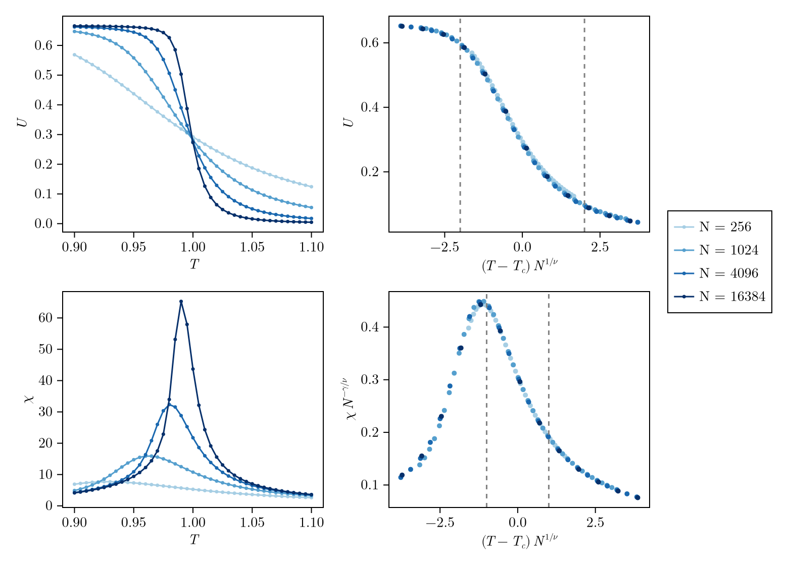

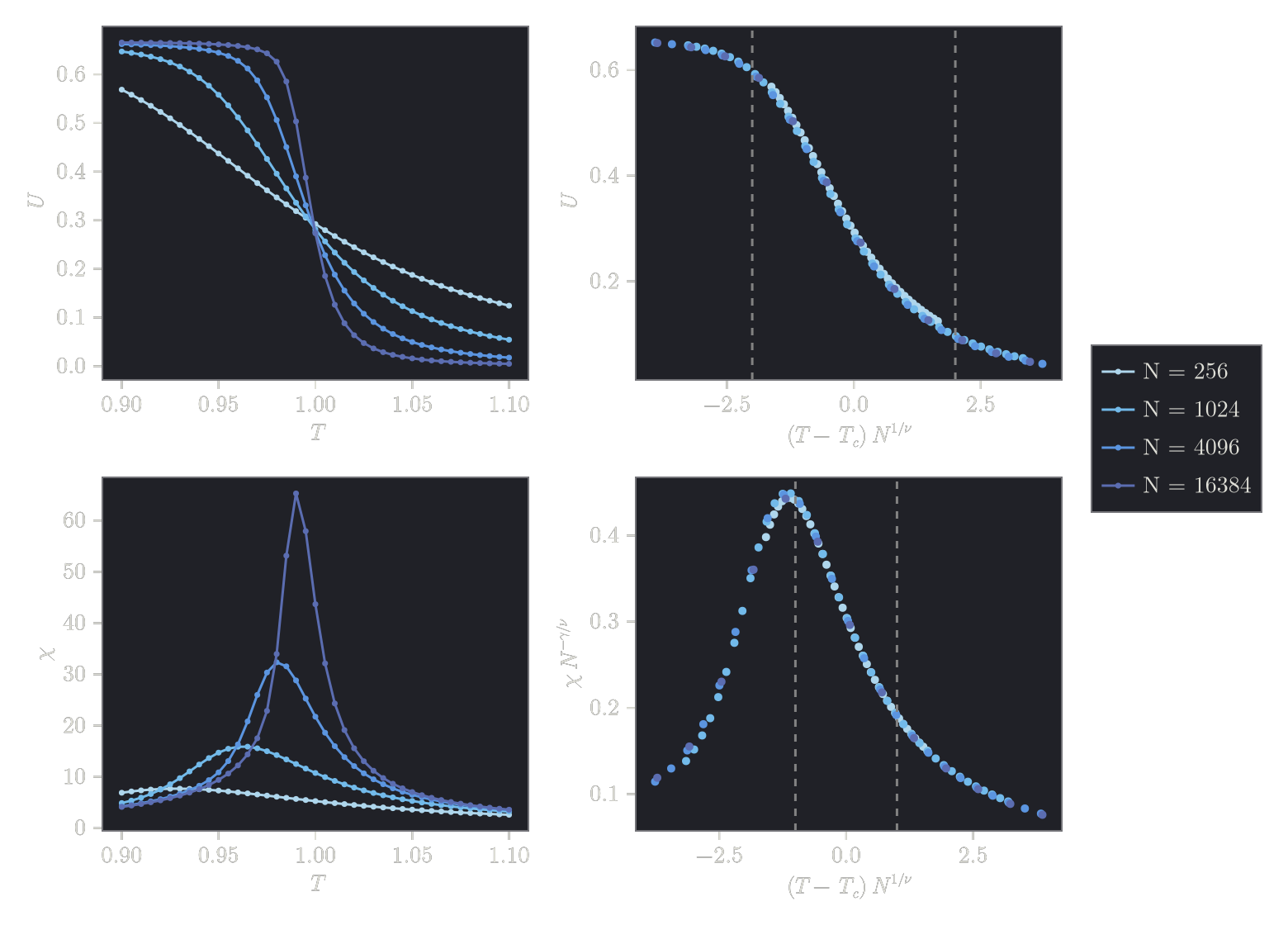
Exact data are not free of errors

Both fits agree with  ,   and   to within two to three errors, but not exactly, although the data have no noise. The errors here measure the corrections to scaling, which decay as in this model: the scaling form is only the leading term for large . As in the percolation example, larger systems or fewer small ones reduce this bias.