2D Ising model

The ferromagnetic Ising model on the square lattice is the textbook example of a continuous phase transition, and its critical parameters are known exactly:

We determine them from Monte Carlo data for   at 81 temperatures between 1.5 and 3.5. The data ship with the repository of ScalingCollapse.jl (in test/testdata), so the code below runs as it is.

The data

using ScalingCollapse
using HDF5

file = joinpath(pkgdir(ScalingCollapse), "test", "testdata", "IsingMonteCarlo.h5")
Ts, Ls, binder, M, chi = h5open(file) do h
    read(h, "Ts"), read(h, "Ls"), read(h, "binder"), read(h, "M_abs_mean"), read(h, "susceptibility")
end
size(binder)

(81, 4)

Every observable is a matrix with one column per system size and one row per temperature; ScalingProblem recognizes the orientation from the number of sizes. To compare raw and rescaled data throughout this page, we use a small plotting function. It shows the rescaled data only within window, and marks the window dx of the fit with dashed lines.

using CairoMakie

function plot_collapse(sp; xlabel, ylabel, xlabel_scaled, ylabel_scaled, window=(-Inf, Inf))
    colors = cgrad(:Blues)[range(0.35, 1.0; length=length(sp.data))]
    fig = Figure(size=(780, 320))
    ax1 = Axis(fig[1, 1]; xlabel, ylabel, title="data")
    ax2 = Axis(fig[1, 2]; xlabel=xlabel_scaled, ylabel=ylabel_scaled, title="collapse")
    xs, ys, _, Ls = scaled_data(sp)
    for (i, d) in enumerate(sp.data)
        scatterlines!(ax1, d.xs, d.ys; color=colors[i], markersize=5, label="L = $(Ls[i])")
        inside = window[1] .<= xs[i] .<= window[2]
        scatter!(ax2, xs[i][inside], ys[i][inside]; color=colors[i], markersize=7)
    end
    vlines!(ax2, filter(isfinite, sp.dx); color=:gray, linestyle=:dash)
    Legend(fig[1, 3], ax1)
    return fig
end

Binder cumulant

The Binder cumulant    is dimensionless: at it does not depend on , and close to it follows   . Only the x axis needs rescaling, so we use the preset :x:

sp_binder = ScalingProblem(Ts, binder, Ls;
    sf=ScalingFunction(:x; p_names=["T_c", "nu"]),
    p_space=[2.0:0.02:2.6, 0.5:0.05:1.5],
    dx=[-2.0, 2.0],
)

ScalingProblem
    Scaling function:
        x -> (x - T_c) * L^(1/nu)
        y -> y
    Optimal parameters:
        T_c = 2.268292508881059 ± 0.0017732093354786754
        nu = 0.9981387418335177 ± 0.034960309522727384
    Optimization interval dx:
        -2.0 < x < 2.0
    Searched parameter space:
        T_c ∈ 2.0:0.02:2.6
        nu ∈ 0.5:0.05:1.5

Both parameters agree with the exact values within their errors.

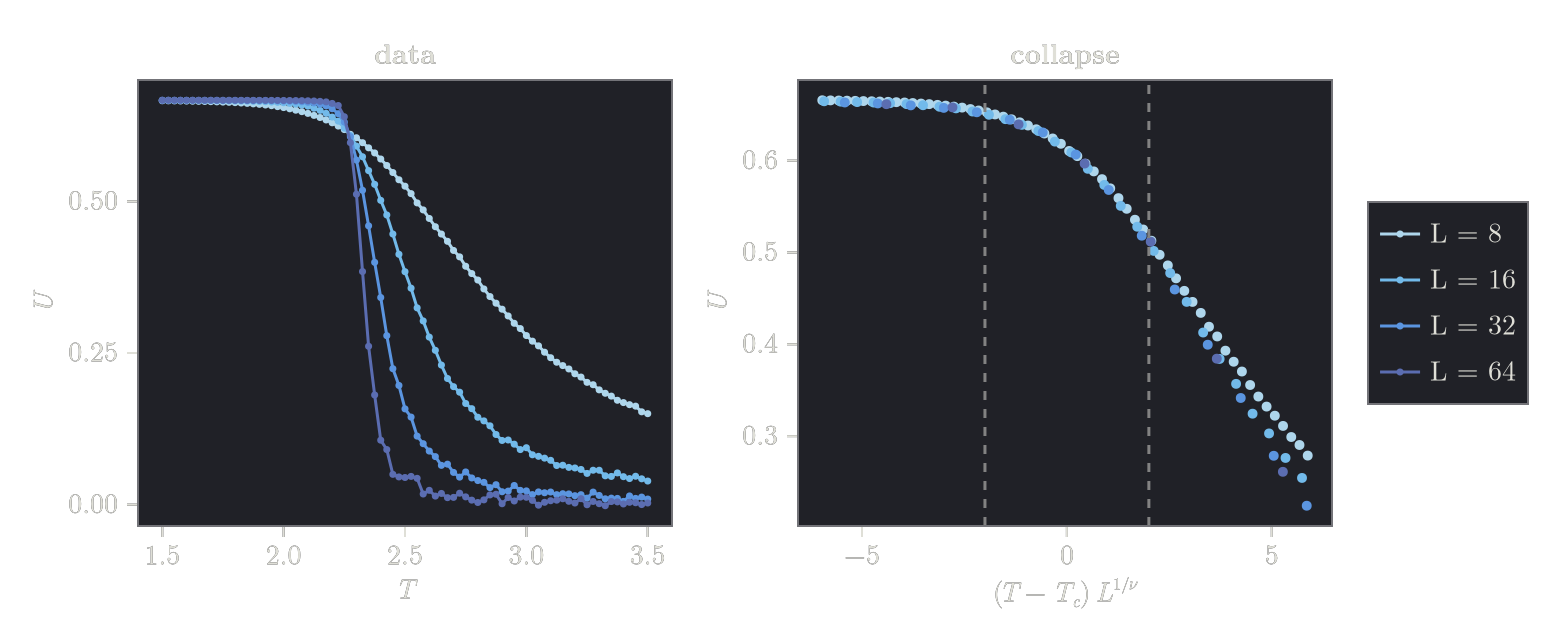
plot_collapse(sp_binder; xlabel=L"T", ylabel=L"U",
    xlabel_scaled=L"(T - T_c)\,L^{1/\nu}", ylabel_scaled=L"U", window=(-6, 6))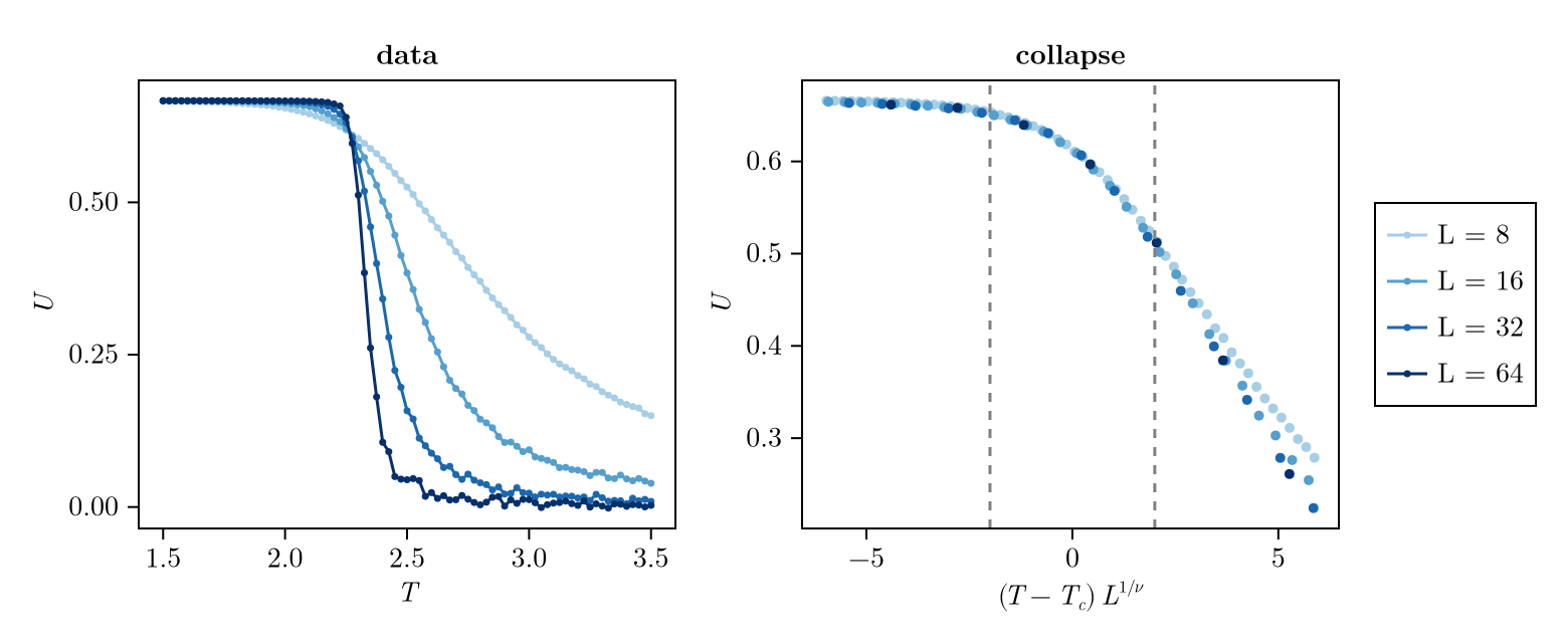

Fixing ν

Since   is known, we can fix it and fit only , which reduces its error:

sp_binder_nu = ScalingProblem(Ts, binder, Ls;
    sf=ScalingFunction(:x; p_names=["T_c", "nu"], nu=1),
    p_space=[2.0:0.01:2.6],
    dx=[-2.0, 2.0],
)

ScalingProblem
    Scaling function:
        x -> (x - T_c) * L^(1/nu)
        y -> y
    Fixed parameters:
        nu = 1.0
    Optimal parameters:
        T_c = 2.2682312011718744 ± 0.00117889882952889
    Optimization interval dx:
        -2.0 < x < 2.0
    Searched parameter space:
        T_c ∈ 2.0:0.01:2.6

Magnetization

The order parameter vanishes at as  , so is a function of   only. This is the preset :xy, which rescales y as :

sp_mag = ScalingProblem(Ts, M, Ls;
    sf=ScalingFunction(:xy; p_names=["T_c", "nu", "beta"]),
    p_space=[2.1:0.02:2.4, 0.6:0.1:1.4, 0.05:0.025:0.3],
    dx=[-2.0, 2.0],
)

ScalingProblem
    Scaling function:
        x -> (x - T_c) * L^(1/nu)
        y -> y * L^(beta/nu)
    Optimal parameters:
        T_c = 2.2686335809650053 ± 0.002828404649752289
        nu = 0.95126759671457 ± 0.027780180222311372
        beta = 0.11574695917101487 ± 0.006722664904079725
    Optimization interval dx:
        -2.0 < x < 2.0
    Searched parameter space:
        T_c ∈ 2.1:0.02:2.4
        nu ∈ 0.6:0.1:1.4
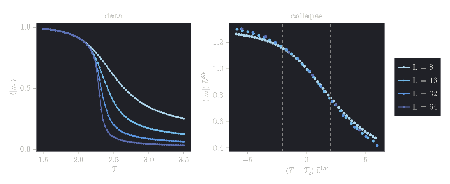
        beta ∈ 0.05:0.025:0.3

plot_collapse(sp_mag; xlabel=L"T", ylabel=L"\langle |m| \rangle",
    xlabel_scaled=L"(T - T_c)\,L^{1/\nu}", ylabel_scaled=L"\langle |m| \rangle\, L^{\beta/\nu}",
    window=(-6, 6))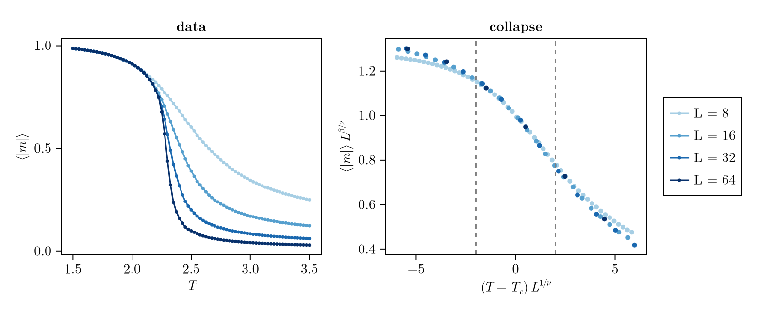

Susceptibility

The susceptibility diverges as  . The preset :xny rescales y as , so that comes out positive:

sp_chi = ScalingProblem(Ts, chi, Ls;
    sf=ScalingFunction(:xny; p_names=["T_c", "nu", "gamma"]),
    p_space=[2.1:0.02:2.4, 0.6:0.1:1.4, 1.2:0.1:2.2],
    dx=[-2.0, 2.0],
)

ScalingProblem
    Scaling function:
        x -> (x - T_c) * L^(1/nu)
        y -> y * L^(-gamma/nu)
    Optimal parameters:
        T_c = 2.2693211452470483 ± 0.004526597481725415
        nu = 1.0399074636804229 ± 0.0631116054941655
        gamma = 1.8387856157550522 ± 0.14025512603398332
    Optimization interval dx:
        -2.0 < x < 2.0
    Searched parameter space:
        T_c ∈ 2.1:0.02:2.4
        nu ∈ 0.6:0.1:1.4
        gamma ∈ 1.2:0.1:2.2

plot_collapse(sp_chi; xlabel=L"T", ylabel=L"\chi",
    xlabel_scaled=L"(T - T_c)\,L^{1/\nu}", ylabel_scaled=L"\chi\, L^{-\gamma/\nu}",
    window=(-6, 6))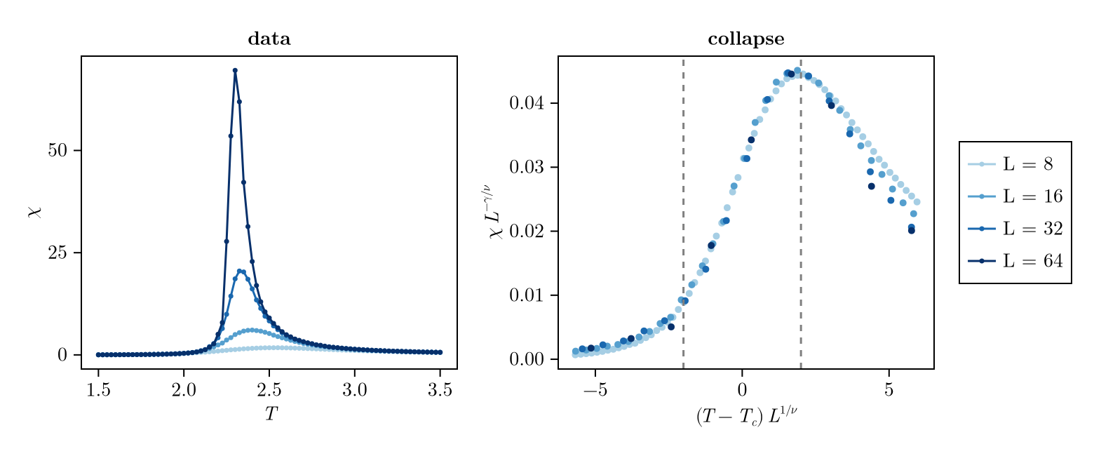

Summary

exact = Dict("T_c" => 2 / log(1 + sqrt(2)), "nu" => 1.0, "beta" => 1 / 8, "gamma" => 7 / 4)
for (name, sp) in ("Binder" => sp_binder, "Binder, ν = 1" => sp_binder_nu,
    "magnetization" => sp_mag, "susceptibility" => sp_chi)
    println(name)
    for (p, v, σ) in zip(ScalingCollapse.scaled_p_names(sp.sf), sp.optimal_ps, sp.optimal_ps_error)
        println("    ", rpad(p, 6), round(v; digits=4), " ± ", round(σ; digits=4),
            "   (exact ", round(exact[p]; digits=4), ", ", round(abs(v - exact[p]) / σ; digits=1), "σ)")
    end
end

Binder
    T_c   2.2683 ± 0.0018   (exact 2.2692, 0.5σ)
    nu    0.9981 ± 0.035   (exact 1.0, 0.1σ)
Binder, ν = 1
    T_c   2.2682 ± 0.0012   (exact 2.2692, 0.8σ)
magnetization
    T_c   2.2686 ± 0.0028   (exact 2.2692, 0.2σ)
    nu    0.9513 ± 0.0278   (exact 1.0, 1.8σ)
    beta  0.1157 ± 0.0067   (exact 0.125, 1.4σ)
susceptibility
    T_c   2.2693 ± 0.0045   (exact 2.2692, 0.0σ)
    nu    1.0399 ± 0.0631   (exact 1.0, 0.6σ)
    gamma 1.8388 ± 0.1403   (exact 1.75, 0.6σ)

All parameters lie within about two errors of the exact values. The largest deviation, from the magnetization, comes from corrections to scaling, which are largest for the smallest size,  . The data have no error bars, so the errors are the default profile widths (see Error analysis).